Some informal notes on the methods implemented in `wgd`¶

Author:	Arthur Zwaenepoel

Contents

Some informal notes on the methods implemented in wgd

Introduction ¶

wgd is a python package and command line suite for analyzing ancient whole genome duplications (WGDs) in genomic data sets. The main focus of wgd is on the construction of whole paranome (the collection of all duplicate genes in a genome) K_S distributions, but it also provides tools for the inference of intragenomic synteny and anchor points as well as downstream analyses and visualizations of whole paranome K_S distributions. On this page we provide some background information and informal explanations about the main functionality and methods, namely the inference of these so-called K_S distributions. This is not a tutorial on how to use wgd, for that, please have a look at the command line interface or at the supplementary material of our Bioinformatics paper.

What is a K_S distribution?¶

K_S, also called dS, denotes the synonymous distance between two protein- coding DNA sequences (CDS), where synonymous distance means the expected number of synonymous substitutions per synonymous site. A K_S estimate for any two coding sequences can be acquired in two main ways, (1) by means of heuristic counting methods such as the method of Nei & Gojobori (1986) or (2) by using Markov models of codon substitution with Maximum-likelihood (ML) estimation algorithms. The latter methods are most commonly used nowadays, and trace back to the pioneering work of Goldman & Yang (1994) and Muse & Gaut (1994). For more information on the estimation of pairwise synonymous distances, we refer to the wonderful textbooks on molecular evolution authored by professor Ziheng Yang (e.g. Chapter 2 in Yang 2006).

Since synonymous substitutions are presumed to have largely negligible effects on fitness, they are commonly regarded as neutral. Therefore we expect the synonymous distance between two protein coding sequences to increase with time in a stochasti clock like fashion. It is therefore assumed that K_S can serve as a proxy for time, and that a larger K_S value indicates an older divergence time between two sequences.

A whole paranome K_S distribution is nothing more than the distribution of all K_S estimates for all inferred duplication events in the genome of some species. It therefore serves as a proxy for the distribution of the divergence times of all duplication events that have left a trace in the genome of interest. Under the assumption of a constant gene duplication rate and a constant rate of loss of duplicated copies, such a distribution is expected to show an exponential decay shape (Lynch & Conery 2000, Lynch 2007), which is the result of a quasi- equilibrium linear birth-death process. A WGD event entails the duplication of all gene copies in the genome at some point in time (i.e. the polyploidization event) and subsequent massive loss or divergence of duplicated copies in a relatively short time frame (i.e. the rediploidization phase). This process of WGD followed by rediploidization is expected to leave a large number of duplication events with similar divergence times (and hence similar K_S values) that can be traced back in the extant genome of interest. As a result a WGD is expected to leave a peak signature in the K_S distribution that cannot be explained by constant rate small-scale duplication as in the model of Lynch & Conery.

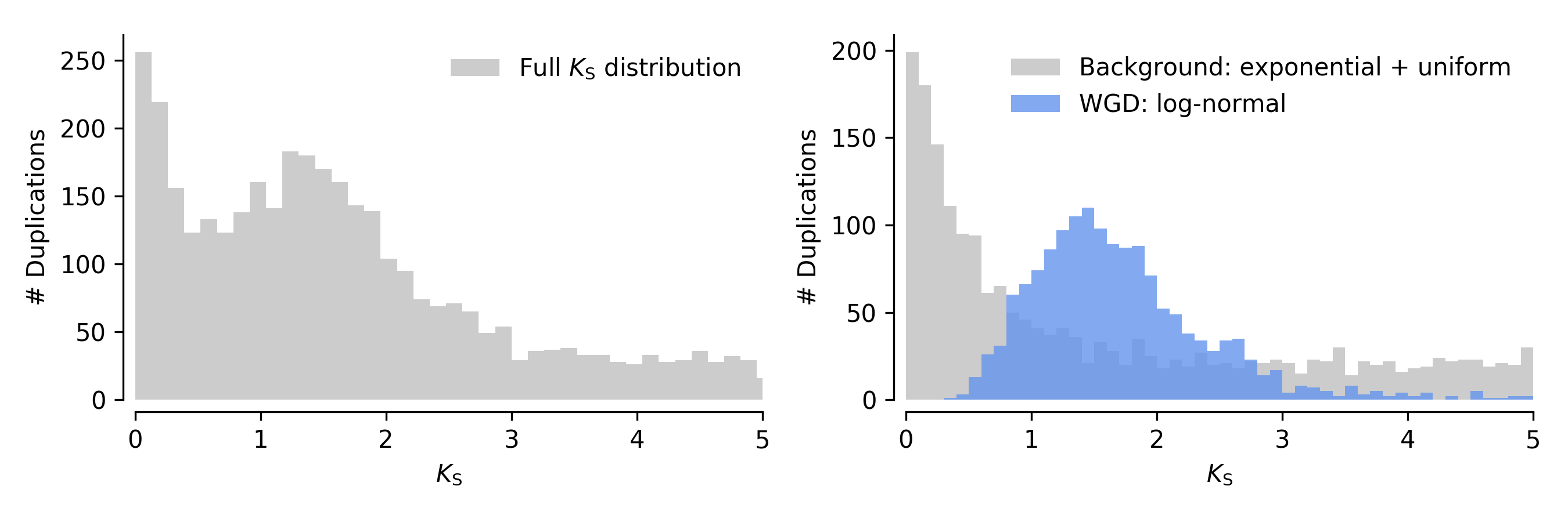
As a side note, we note that if we assume synonymous substitution is a Poisson process, and the synonymous substitution rate is Gamma distributed across gene families, this WGD peak signature is expected to follow a negative binomial distribution in the ditribution of numbers of synonymous substititions (which is not the same as K_S distribution). In the K_S distribution, this would translate to a peak which has a distribution with positive skew, which we could approximate by a Gamma or Log-Normal distribution. These considerations are important for mixture modeling. An ad hoc illustration of such a hypothetical K_S distribution is shown below. The left plot shows the full K_S distribution, whereas the right plot shows the decomposition into the background signature from the continuous birth, death and fixation of small-scale duplicates (gray) and the WGD signature (in blue, here modeled as a log-normal distribution).

How is the K_S distribution computed in `wgd`?¶

While the basic idea seems simple enough, constructing a K_S distribution is a rather involved business. This is the main reason why we released wgd, to make this seemingly simple approach actually simple to perform. Below we elaborate on the main steps undertken in a K_S distribution construction.

Inferring duplicates ¶

First, we need to infer the duplicate genes in the genome. To this end, commonly employed homolog clustering approaches are used in wgd mcl. Since we are however not interested in multi-species gene families, these homolog clustering methods are used only within a particular genome of interest. wgd mcl clusters genes into paralogous families (where all genes are paralogous to each other, i.e. diverged after some duplication event) by

Doing an all-versus-all Blastp similarity search
Constructing a sequence similarity graph based on the Blastp results
Finding clusters in the graph by means of an unsupervised approach using the Markov Clustering algorithm (MCL, Vandongen 2000).

For more information on these approaches, please consult literature on homolog clustering (e.g. OrthoMCL, OrthoFinder), but bear in mind that we are only concerned with within genome homolog clusters, i.e. paralogous gene families.

Calculating pairwise Ks values ¶

For every paralogous family we inferred, we first construct a multiple sequence alignment (MSA) using standard practices (in wgd ksd you can choose between MUSCLE, MAFFT and PRANK for alignment). Alignments are constructed at the amino acid level as these can be more reliable, and are backtranslated to nucleotide sequences to obtain a codon-alignment.

Now that we have our paralogous gene families and MSAs, we can compute for every pair in the family the synonymous distance, K_S. To this end wgd ksd uses the codeml program from the PAML package. codeml has tons of parameter settings and algorithmic options, and those used in wgd ksd will not be reiterated here but can be found in the supplement to Zwaenepoel & Van de Peer (2018) or Vanneste et al. (2013). In general, the settings are set such that they do a good job at estimating pairwise K_S values reliably by maximum likelihood.

Calculating Ks estimates for duplication events¶

Note that after the previous step step we have n(n-1)/2 pairwise K_S estimates for a paralogous family with n genes, whereas what we really want is Ks estimate for each duplication event in the family. If multiple duplications happened, we will have multiple redundant K_S estimates for internal duplication nodes in the gene family tree. To see this, have a look at the figure below, where a paralogous gene tree is shown, with two marked internal duplication nodes and their respective K_S values.

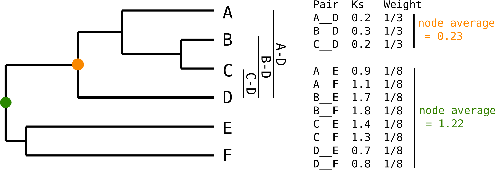
We are interested in the divergence time (approximated by K_S) for the five internal nodes of this tree, whereas what we really have is 6x5/2= 15 K_S estimates between all pairs of leaves. As is clear from this figure, we have 3 redundant estimates for the orange node, whereas we have 8 redundant estimates for the green node. We can correct for this redundancy by either averaging K_S values for each node (or taking some other summary statistic like the median), or by computing a weight for every K_S value. (see also next section).

However, to do this we of course need the tree, therefore wgd ksd will compute for every paralogous gene family a phylogenetic tree after calculating the pairwise K_S values to do redundancy correction (either by node-averaging or node-weighting, see below). In wgd ksd one can choose between three options to construct this tree, either average linkage clustering of K_S values (which is fast but somewhat crude), approximate ML tree inference using FastTree (Price et al.) or ML tree inference using PhyML (which is obviously the slowest option).

After the tree is computed wgd ksd will write for every pair the Ks estimate, some alignment statistics, the node in the tree for which the Ks value provides a divergence estimate, the gene family, the various distance estimates (K_S, K_A and ω) and the weights computed without filtering out outliers and with filtering out outliers (see below).

Visualizing a K_S distribution ¶

If all goes well, wgd ksd will compute a K_S distribution which looks somewhat like this (where I have omitted lots of columns that are not really of interest currently):

                            Family      Ks         Node     WeightOutliersExcluded
AT3G11180__AT5G05600        GF_000093   0.7679     23.0     1.00
AT2G38240__AT5G05600        GF_000093   1.9122     25.0     0.33
AT2G38240__AT3G11180        GF_000093   2.5219     25.0     0.33
AT5G08640__AT5G63580        GF_000093   1.3265     30.0     0.20
...                         ...

Now, simply plotting a histogram of the resulting K_S values will of course be flawed, since we will plot all redundant estimates with equal weight, and since older duplication events will have more pairwise estimates, this may artificially amplify the signal of old duplication events.

There are two main approaches to overcome this, already noted in the previous section. The first is node-averaging, where one computes a summarized K_S value for each node. This is easily performed using built-in functions to work with data frames in R or Python. This approach obviously throws away the information in the individual pairwise estimates and only uses the summarized value in subsequent analysis. The second approach is node-weighting, where one computes a weight for every pairwise estimate, and adds every single estimate to the histogram but with some weighted based on the number of redundant etimates. Such an approach does not throw away the information in individual estimates, but is trickier to work with in subsequent analyses such as Kernel density estimation (KDE) or Gaussian mixture modeling (GMMs). Weighted histograms can be plotted both in ggplot2 in R and matplotlib in Python.

It is important to be aware that different filters on the K_S range, will cause the weights to change. Indeed, if some pairwise estimate is filtered out, because of some filtering riterion, the number of K_S estimates will change for that particular duplication event. This is exactly the difference between the WeightOutliersIncluded column and WeightOutliersExcluded column, where the weights in the latter column are based on the number of pairwise estimates after filtering, whereas the former has weights based on the number of pairwise estimates before filtering. It is does important to recompute the weights when different filtering riteria are used. The tools in wgd will always do this, but it is important to keep in mind when analyzing the dat yourelf in R or some other statistical/plotting environment.

Note that wgd ksd by default outputs node-weighted histograms, whereas node-averaged histograms can be generated using wgd viz. The mixture modeling and KDE methods in wgd mix and wgd kde use node-averaged histograms for modeling purposes.

Downstream analyses ¶

Downstream analyses consist mainly of fitting different models to a K_S distribution, which could be KDEs, or mixture models. For more information on mixture modeling of K_S distributions, we refer to A note on mixture models for KS distributions.