Mixture modeling
The mixture modeling features of wgd use the sci-kit learn
(better known as sklearn library).
A note on mixture models for KS distributions
Mixture models have been employed frequently to study WGDs with KS distributions. Under several basic molecular evolutionary assumptions, the peak in the KS distribution caused by a WGD is expected to show a distribution with positive skew, which can be reasonably well approximated by a log-normal distribution. Fitting mixtures of log-normal components and statistical evaluation of different model fits is therefore a reasonable strategy to locate WGD-derived peaks in a KS distribution.
However, mixture models are known to be prone to overfitting and overclustering, and this is especially true for KS distributions where we have a lot of data points (see e.g. Tiley et al. (2018) for a recent study on mixture models for WGD inference). Therefore, we do not advise to use mixture models as formal statistical tests of multiple WGD hypotheses. We mainly regard mixture models as providing a somewhat more formal representation of what a researcher understands as a ‘peak’ giving evidence for a WGD. Additionaly, mixture models allow to obtain an estimate for the mean and variance of hypothesized WGD peaks. Also, mixture models allow a means of selecting paralogous pairs that are derived from a hypothesized WGD using quantitative measures. That is, given a fitted mixture model which we regard as representing our hypothesis of ancient WGDs, we can isolate those gene pairs that belong with, say, 95% probability to the component under the model. This is likely a preferable approach compared to applying arbitrary cut-offs based on visual inspection.
A note on the practical difference between the BGMM and GMM method
For algorithmic and theoretical details, we refer to http://scikit-learn.org/stable/modules/classes.html#module-sklearn.mixture. Here we give a pragmatic description. Again we stress that mixture modeling results should not be taken as evidence for WGD as such, and should also be interpreted with caution (see above)!
The GMM method
When using the GMM method, model selection proceeds by evaluating relative model
fit using the Bayesian or Akaike information criterion ([B/A]IC). Comparison of
AIC values across models can be used to assess which model fits the data best
according to the AIC. As an example, consider the output of wgd mix:
AIC assessment:
min(AIC) = 25247.22 for model 4
Relative probabilities compared to model 4:
    /                          \
    |      (min(AIC) - AICi)/2 |
    | p = e                    |
    \                          /
.. model   1: p = 0.0000
.. model   2: p = 0.0000
.. model   3: p = 0.0000
.. model   4: p = 1.0000
.. model   5: p = 0.0005
The p computed by the formula shown in this output can be interpreted as proportional to the probability that model i minimizes the information loss. More specifically in this example, model 5 is 0.0005 as probable to minimize the expected information loss as model 4. In this case the AIC clearly supports the 4 component model.
The BIC based model selection procedure is analogous. For every model fit we calculate the BIC value and we record the difference with the minimum BIC value (this is the Delta BIC value). If we interpret Delta BIC values as Bayes factors, we can again perform model selection:
Delta BIC assessment:
min(BIC) = 25327.22 for model 4
.. model   1: delta(BIC) =  3970.57 (    >10: Very Strong)
.. model   2: delta(BIC) =  1758.68 (    >10: Very Strong)
.. model   3: delta(BIC) =    38.39 (    >10: Very Strong)
.. model   4: delta(BIC) =     0.00 (0 to  2:   Very weak)
.. model   5: delta(BIC) =    37.17 (    >10: Very Strong)
Where ( >10: Very Strong) denotes very strong support of model 4 over
another model. These results confirm the results of the AIC values.
The BGMM Method
The BGMM method uses a variational Bayes algorithm to fit infinite Gaussian mixture models using a Dirichlet process (DP) prior on the mixture components. This is a Bayesian nonparametric clustering approach and does not require, in principle to select an a priori fixed number of components. In theory, for an infinite GMM with the DP prior, the more data points the more clusters one should obtain, and the method is theoretically not really geared towards determining the ‘true’ number of components in the distribution.
However, the method can also be regarded from a regularization perspective, where a prior distribution on the component weights can be used to constrain model flexibility. That is, for particular choices of the hyperparameter governing the DP prior (denoted as gamma), the model fitting procedure will allow more or less components to be active in the mixture. For low values of gamma, the model fitting procedure effectively penalizes the number of high weight components in the mixture. In wgd we provide plots of the mixture with associated weights for each component such that the user can visually discern whether some component is active or inactive (negligible weight) in the mixture.
For example, using the same distribution as in the previous paragraph, a mixture with 5 components looks like this:
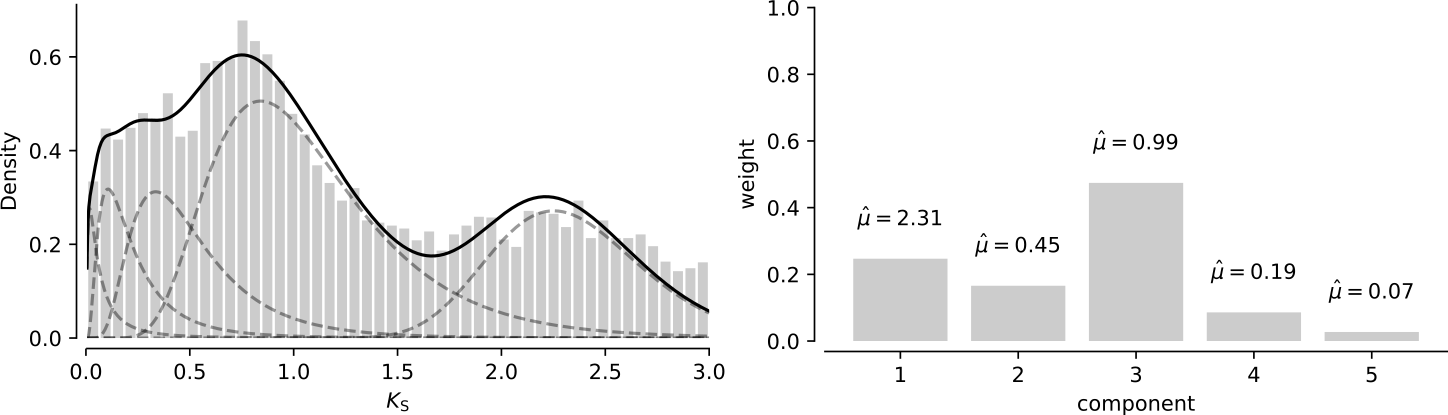
Here we see that the fifth component with mean 0.07 has negligible weight compared to the other components in the mixture, which agrees with the results from above.
Reference
Copyright (C) 2018 Arthur Zwaenepoel
This program is free software: you can redistribute it and/or modify it under the terms of the GNU General Public License as published by the Free Software Foundation, either version 3 of the License, or (at your option) any later version.
This program is distributed in the hope that it will be useful, but WITHOUT ANY WARRANTY; without even the implied warranty of MERCHANTABILITY or FITNESS FOR A PARTICULAR PURPOSE. See the GNU General Public License for more details.
You should have received a copy of the GNU General Public License along with this program. If not, see <http://www.gnu.org/licenses/>.
Contact: arzwa@psb.vib-ugent.be
-
wgd.modeling.filter_group_data(df, aln_id=0, aln_len=300, aln_cov=0, min_ks=0, max_ks=5, weights_outliers_included=False)¶ Filter a Ks data frame for modling purposes.
Parameters: - df – data frame
- aln_id – alignment identity threshold
- aln_len – alignment length threshold
- aln_cov – alignment coverage threshold
- min_ks – minimum Ks value
- max_ks – maximum Ks value
- weights_outliers_included – boolean, adapt weights when removing outliers
Returns: filtered data frame
-
wgd.modeling.fit_bgmm(X, n1, n2, gamma=0.001, max_iter=100, n_init=1, **kwargs)¶ Compute Bayesian Gaussian mixture
Parameters: - X – data frame (log transformed Ks values)
- n1 – minimum number of components
- n2 – maximum number of components
- gamma – inverse of regularization strength
- max_iter – maximum number of iterations
- n_init – number of k-means initializations
- kwargs – other keyword args for GaussianMixture
Returns: models
-
wgd.modeling.fit_gmm(X, n1, n2, max_iter=100, n_init=1, **kwargs)¶ Compute Gaussian mixtures for different numbers of components
Parameters: - X – data frame (log transformed Ks values)
- n1 – minimum number of components
- n2 – maximum number of components
- max_iter – maximum number of iterations
- n_init – number of k-means initializations
- kwargs – other keyword args for GaussianMixture
Returns: models, bic, aic, best model
-
wgd.modeling.get_array_for_mixture(df)¶ Get an array of log transformed Ks values.
Parameters: df – data frame Returns: array
-
wgd.modeling.get_component_probabilities(df, model)¶ Get paralogs from a mixture model component.
Parameters: - df – Ks distribution pandas data frame
- model – mixture model
Returns: data frame
-
wgd.modeling.inspect_aic(aic)¶ Evaluate the Akaike information criterion results for mixture models.
Parameters: aic – AIC values
-
wgd.modeling.inspect_bic(bic)¶ Evaluate the BIC values
Parameters: bic – BIC values
-
wgd.modeling.plot_aic_bic(aic, bic, min_n, max_n, out_file)¶ Plot AIC and BIC curves
Parameters: - aic – aic values
- bic – bic values
- out_file – output file
Returns: nada
-
wgd.modeling.plot_all_models_bgmm(models, data, l, u, bins, out_file)¶ Plot a bunch of BGMMs.
Parameters: - models – list of GMM model objects
- data – Ks array
- l – lower Ks limit
- u – upper Ks limit
- bins – number of histogram bins
- out_file – output file
Returns: nada
-
wgd.modeling.plot_all_models_gmm(models, data, l, u, bins, out_file)¶ Plot a bunch of GMMs.
Parameters: - models – list of GMM model objects
- data – Ks array
- l – lower Ks limit
- u – upper Ks limit
- bins – number of histogram bins
- out_file – output file
Returns: nada
-
wgd.modeling.plot_bars_weights(model, ax)¶ Plot Component weights
Parameters: - model – model
- ax – figure ax
Returns: ax
-
wgd.modeling.plot_mixture(model, data, ax, l=0, u=5, color='black', alpha=0.2, log=False, bins=25, alpha_l1=1)¶ Plot a mixture model. Assumes a log-transformed model and data and will back-transform.
A common parametrization for a lognormal random variable Y is in terms of the mean, mu, and standard deviation, sigma, of the unique normally distributed random variable X such that exp(X) = Y. This parametrization corresponds to setting s = sigma and scale = exp(mu).
So since we fit a normal mixture on the logscale, we can get the lognormal by setting scale to np.exp(mean[k]) and s to np.sqrt(variance[k]) for component k.
Parameters: - model – model object
- data – data array
- ax – figure ax
- l – lower Ks limit
- u – upper Ks limit
- color – color for histogram
- alpha – alpha value
- log – plot on log scale?
- bins – number of histogram bins
- alpha_l1 – alpha value for mixture lines
Returns: ax
-
wgd.modeling.plot_probs(m, ax, l=0.0, u=5, ylab=True)¶ Plot posterior component probabilities
Parameters: - m – model
- ax – figure ax
- l – lower Ks limit
- u – upper Ks limit
- ylab – plot ylabel?
Returns: ax
-
wgd.modeling.reflect(data)¶ Reflect an array around it’s left boundary
Parameters: data – np.array Returns: np.array
-
wgd.modeling.reflected_kde(df, min_ks, max_ks, bandwidth, bins, out_file)¶ Perform Kernel density estimation (KDE) with reflected data. The data frame is assumed to be grouped already by ‘Node’.
Parameters: - df – data frame
- min_ks – minimum Ks value (best is to use 0, for reflection purposes)
- max_ks – maximum Ks value
- bandwidth – bandwidth (None results in Scott’s rule of thumb)
- bins – number of histogram bins
- out_file – output file
Returns: nada